09 Dec 2025
Notes On Motion Blur Rendering
Introduction
A while ago, I wanted to take a breather from working on cloud and atmosphere rendering for my hobby renderer. I decided to take a stab at motion blur since I had some ideas that I wanted to try out.
Inevitably, I spent way more time on it than I thought I would. I suppose that’s one of the advantages of a hobby project. We can indulge in a topic like this, obsessing over zoomed-in stills of moving objects
for as long as we want without having to justify how much time we’re spending on it.
Anyway, the result is mostly a combination of existing techniques with some tweaks and adjustments to make them fit together.
Nonetheless, I hope this post will prove useful or at least entertaining.
Previous Work
I won’t cover the existing work in much depth. If you want more details on the prior work, just go and read the references. I found all of them to be very approachable. The seminal paper from McGuire et al. [1] is what the other papers are built upon. The high-level idea is to implement motion blur as a post effect, utilizing the scene color, pixel motion vectors and depth. The maximum motion from a screen area is downsampled into a lower resolution and dilated. This produces conservative motion tiles that are used to pick the blur direction. The maximum blur radius is tied to the size of the motion tiles. This ensures that a pixel will always pick up relevant foreground pixels that blur over it. Depth is used to classify samples as background and foreground. Combined with comparing sample and pixel velocity, this is used to classify samples into multiple cases, producing a plausible effect.
The work by Sousa [2] improved performance by simplifying the weight computation and baking velocity into a texture along with depth. In addition, it improved quality by running the filter multiple times. This allowed high-quality results without undersampling while keeping sample counts low.
Jimenez’s work on Call of Duty [3] focused on improving gradient quality. It introduced a new weighing scheme that avoided discontinuities between foreground and background. In addition, it introduced a mirrored reconstruction filter to further reduce discrepancies in the blur. It uses a single pass and nearest-neighbor sampling to avoid leaking. A checkerboard dither is used to hide undersampling artifacts.
Guertin et al. focused on extending the effect to use an additional sampling direction [4]. Since the previous approach only blurs in the dominant motion, it can cause artifacts in screen areas with complex motion, e.g. rotations or separately moving background and foreground.
Goals
My initial implementation was based on the CoD approach. For any further modifications, I wanted to maintain the smooth gradients. The goals were to add sampling in an additional direction to improve visuals under complex motion as in [4] and to fight undersampling using a two-pass approach as in [2]. In addition, to reduce the performance impact of these improvements, I investigated running motion blur at half resolution. This idea isn’t new. It was already proposed in multiple places [5][6]. However, they did not go into a lot of detail, and I wanted to ensure that there is no leaking and to retain full resolution background color on pixels where a blurry foreground is on top of a sharp background.
Baseline
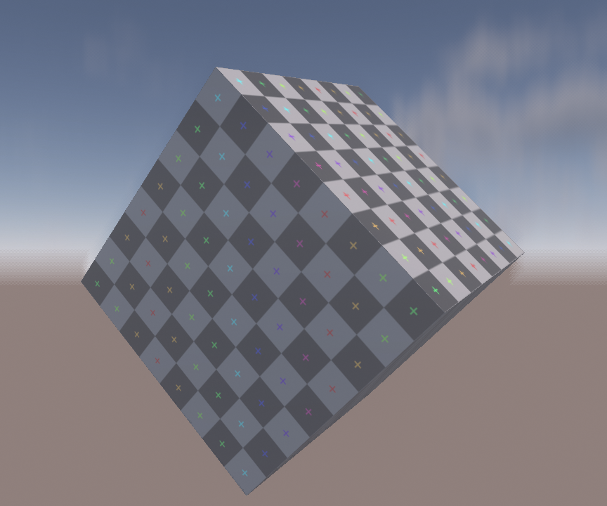
As mentioned before, my first version was a straightforward implementation of the CoD approach [3]. The blur formulation combined with the mirror filter provides smooth gradients.
Leaking is avoided by using nearest-neighbor filtering. The color uses a pre-exposed R11G11B10 HDR color format (although RGB9E5 would be preferable if the hardware supports it).
Depth and velocity are packed together into a two-channel 16-bit float texture.
My home setup is getting somewhat dated at this point, so I’m usually just running everything at 1080p.
For this I’m using a motion tile size of 32 pixels. This limits the blur radius, but is sufficient for my use case and resolution. The blur filter uses just 6 samples.
I’m honestly amazed how well this holds when using the checkerboard dither. You can see some artifacts when you freeze the scene and inspect the image in detail. But even then, it’s not too bad.
The blur is dispatched as a fullscreen compute shader. Motion tiles without any movement skip the filtering entirely. Motion tiles where minimum and maximum velocity are close
run a fast path that simply averages the color. This allows us to skip sampling the depth/velocity texture and the ALU for the weight computation. Again, all of this is just following the
CoD presentation.
The only notable details are that the shader that packs depth and velocity together uses wave ops and LDS (if necessary depending on wave size) to compute an initial 8x8 max velocity
downsample [7]. The same shader outputs some additional depth-based data for unrelated rendering features since we are already loading the data.
The motion tiles store 8-bit motion that is normalized to the 32-pixel tile radius.
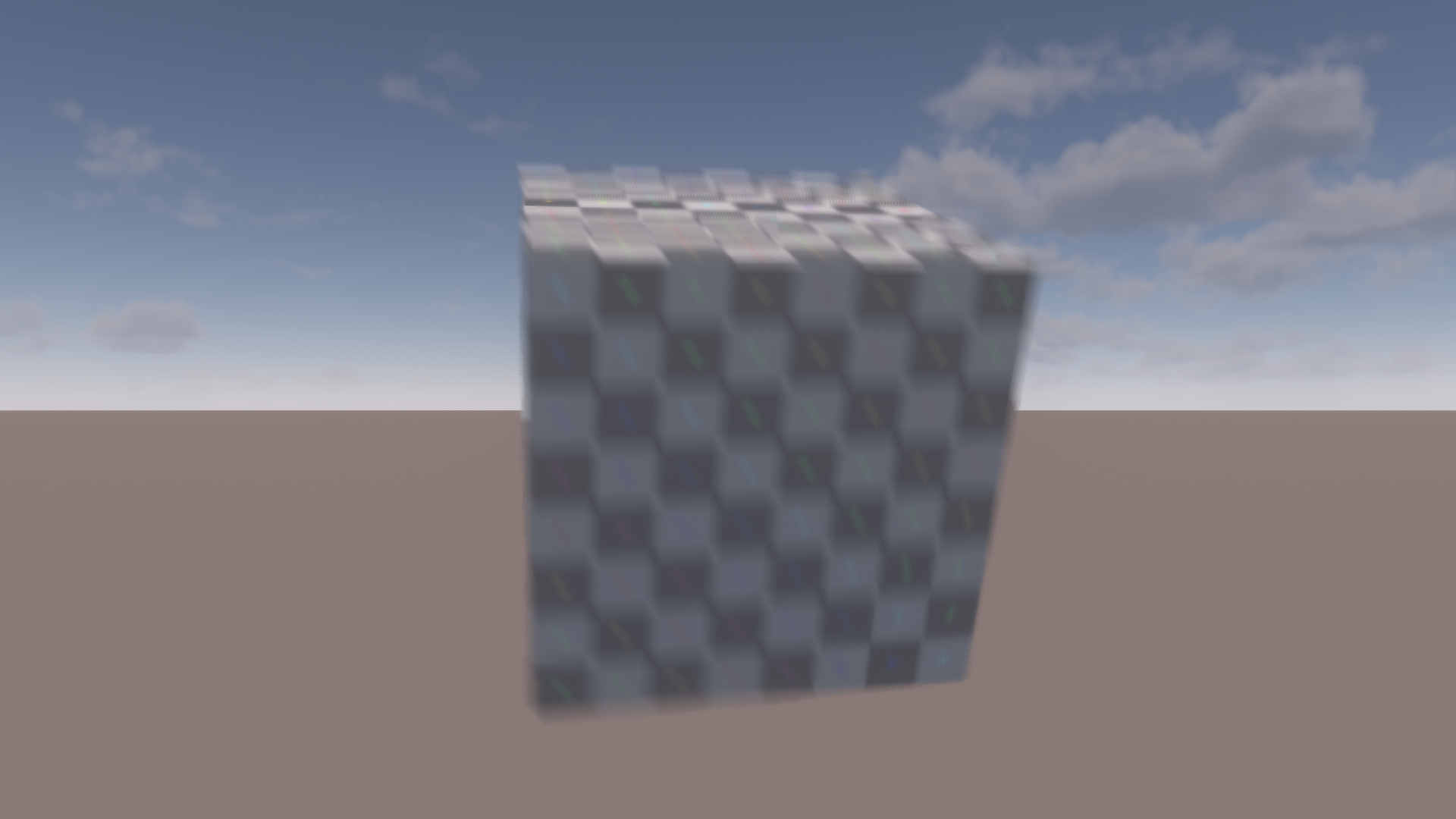
The result in an easy situation with entirely horizontal movement is pretty good. The only obvious downside is the visible dithering in the gradients caused by the low sample count.
I recommend looking at the uncompressed images and at full scale, especially for the later comparisons. Just click on any image to get to its uncompressed PNG version.

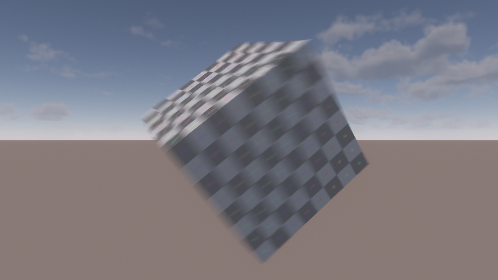
However, the results in a challenging scenario under fast rotation are far less convincing. Borders between motion tiles are clearly visible. This makes it hard to understand the rotation direction from looking at the blur, as well. Lastly, there is some ‘frequency soup’ where sharp and blurred color blends unnaturally, especially visible on the top of the cube. Sharp to blurry transitions should be a transition in blur size and not just a blend between a sharp and fully blurred color.

Let’s check a GPU trace in Nsight to get a quick impression of performance.

Not visible in the screenshots are L1 hit rate at 81% and L2 hit rate at 78%. Cache hit rates are pretty good and the main limiters are L1 and L2 throughputs. This makes sense, since we are taking a lot of samples in a relatively cache-friendly pattern. ALU is clearly underutilized at below 40% SM throughput. I won’t go into much deeper performance analysis here. It might be possible to increase L1 throughput by looking into occupancy or how the samples are scheduled. But I’m not that familiar with Nvidia hardware and the amount of low-level information that Nsight provides is somewhat limited.
The entire dispatch takes ~160us at 1080p on my GTX 1660 ti, running at locked clocks. Not slow, but also not great, considering the quality issues. To get a bit of perspective, the GTX 1660 ti has 5.43 TFLOPs and a bandwidth of 288 GB/s. Those are ~45% and ~50% compared to the Xbox Series X GPU. Obviously, we cannot compare different hardware architectures directly. But if we assume this GPU is around half the speed of a Series X where we might be targeting double the pixel count at 1440p, these numbers should at least be in the same order of magnitude as running a 9th-gen console at a higher, but moderate, resolution.
As a synthetic worst case, I checked what happens when an object covers the majority of the screen and additionally disabling the fast path. This is relatively unrealistic, but results in a cost of ~400us with slightly increased L1 throughput at 78%, SM down to 27% and L2 hit rate slightly increased at 88%.
Separating Background/Foreground
Before we delve into the implementation of the secondary blur direction, I want to share some insight on the background/foreground optimization of the CoD approach. Conceptually, the algorithm accumulates background and foreground colors separately, computes the alpha and blends them. However, it uses an optimization where only a single color is accumulated and at the end the center color is used to balance out the gradient. The alpha value is computed as the percentage of contributing samples. This reduces ALU and register usage. However, something that the presentation does not mention is that this optimization is an approximation and has some edge cases where some artifacts can be visible.
It is true that the optimized version balances out the gradient in terms of the balance between background and foreground. However, consider a scenario with a blurry background and a sharp foreground.
As the blur in the background approaches the sharp foreground, the alpha goes towards zero as more samples hit the sharp foreground. This will increase the contribution of the sharp center color.
What we would want instead is to compute a blurred background color and exclusively use this due to ending up with a foreground alpha of zero. An example where this might be very visible would be an FPS where you
have a fast-moving background under camera motion, while the first-person weapon remains mostly stable in screen-space and therefore sharp. In general, this blend between sharp and blurred colors adds to the
aforementioned ‘frequency soup’.
As a reminder, here are some code snippets for the previous, optimized version that combines background and foreground. Note that most code snippets are slightly adjusted to be more readable in the context of the blog post.
// depthCompare and velocityCompare contain (backgroundWeight, foregroundWeight)
const float sampleWeight = dot(depthCompare, velocityCompare);

// The mirror filter is omitted for simplicity
colorSum += sampleWeight * float4(sampleColor, 1.0);
Then, after all samples have been accumulated, it simply balances the gradient by using the center color. This is equivalent to normalizing the summed color and alpha and interpolating the center color and sum based on the alpha.
colorSum *= sampleCountPerDirectionRcp;
const float3 finalColor = centerColor.rgb * (1.0 - colorSum.a) + colorSum.rgb;
The higher quality option is to simply accumulate foreground and background sums separately.
// Inside the sampling loop
const float2 sampleWeight = depthCompare * velocityCompare;

// Mirror filter is applied here as normal
// ...

backgroundSum += sampleWeight.x * float4(sampleColor[side], 1.0);
foregroundSum += sampleWeight.y * float4(sampleColor[side], 1.0);

// ...
// After the sampling loop
const bool validBackground = backgroundSum.a > 0.0;
const float3 backgroundColor = validBackground ? backgroundSum.rgb / backgroundSum.a : centerColor;

const bool validForeground = foregroundSum.a > 0.0;
const float3 foregroundColor = validForeground ? foregroundSum.rgb / foregroundSum.a : 0.0;

const float foregroundAlpha = sampleCountPerDirectionRcp * foregroundSum.a;
const float3 finalColor = lerp(backgroundColor, foregroundColor, foregroundAlpha);
Let’s take a look at the result:

In this example, the blur on the top of the cube looks much better. Some other areas have been improved as well. Next is an example of the blurry background next to sharp foreground issue. The background is moving vertically. Notice how the horizon line turns sharp in an unnatural way when approaching the cube in the combined version.

The optimization was originally targeted at 8th Gen consoles. Modern GPUs have more registers and tend to offer more ALU in relation to bandwidth and texture throughput. If you are using the approximation, it may be worth checking if it still provides a speedup on your current target hardware. On my GTX 1660 ti, separate background and foreground tracking has a negligible performance impact of around 3-5us.
Second Blur Direction
Using a single blur direction suffers from artifacts in scenarios like rotation and separate background/foreground motion. Let’s demonstrate this with a simple test scene. Here, the cube is blurred horizontally and the background is blurred vertically. In this case, the sharp change in blur direction is very obvious and causes distracting edges in the blur. Dithering the direction between neighboring motion tiles can hide small differences but does very little to help with an extreme case like this.

Guertin et al. use an additional blur direction[4]. They propose using local pixel motion if it has relevant velocity. Otherwise, they fall back to sampling perpendicular to the dominant motion. I found that using the local pixel velocity can cause discontinuities in the blur and is generally unreliable. Sampling in a perpendicular direction can be a poor fit if secondary motion is at an angle, e.g. 45 degrees. In my tests, this scheme tended to waste samples and degraded the gradient quality.
Instead, I compute a secondary direction per motion tile along with the dominant one. The second direction uses an additional weight based on the angle to the primary direction. I found a simple directional weight based on the dot product between the directions to be sufficient. We take the absolute value of the dot product since we blur in both directions. Squaring the result skews the weight a bit more towards larger differences in angle.
float computeSecondaryMotionWeight(float2 primaryMotion, float2 sampleMotion)
{
    const float result = 1 - abs(dot(normalizeSafe(primaryMotion), normalizeSafe(sampleMotion)));
    return result * result;
}
As mentioned before, an initial 8x8 motion is computed inside a compute shader that outputs various depth/motion related data.
Then a second shader picks the dominant direction of four 8x8 tiles to assemble the initial 32x32 tiles. A final pass then dilates the tiles.
The second direction is simply computed at each step by using the intermediate primary motion results. This is technically not as accurate as computing the primary direction first in its entirety and computing
the secondary direction afterwards. However, it avoids the overhead of additional passes and rereading the same data. The results were good enough in my test cases, but your mileage may vary.
Once we have the second blur direction, we have to address weighing of samples and combining both directions. The weighing is very similar to what the paper proposes[4]. We add a term that compares the direction of the sample/center motion to the blur direction using a simple dot product. Note that the weight is applied before the mirror filter.
float2 computeMotionWeights(float2 sampleMotion, float2 samplingDirection, float2 centerMotion)
{
    const float2 weights = abs(float2(
        dot(normalizeSafe(samplingDirection), normalizeSafe(centerMotion)),
        dot(normalizeSafe(samplingDirection), normalizeSafe(sampleMotion))));

    // Applying an extra pow function tends to look a bit better in challenging situations
    // because it improves the directionality of the blur and avoids an overly 'bloomy' isotropic blur look
    return pow(weights, 3.0);
}

// Inside the sampling loop
float2 sampleWeight = depthCompare * velocityCompare;
sampleWeight *= computeMotionWeights(sampleMotion, samplingDirection, centerMotion);
I experimented with a couple of methods of combining the different sampling directions. In the end, I decided to accumulate the color of both directions into background and foreground together for simplicity
and to reduce ALU and register usage. However, more care needs to be taken for the alpha as that is critical for the gradient quality.
First, I slightly modified the depth weight from the CoD paper so that two pixels that have the same depth are classified as background. This pushes the alpha values out of moving foreground objects.
Then simply taking the maximum alpha of both directions works surprisingly well. This ensures that the dominant gradient remains smooth. The modified code for the depth weights remains straightforward:
float2 computeDepthWeights(float sampleDepth, float centerDepth)
{
#if MB_SECOND_DIRECTION
    // Ensure that same depth is background only.
    // This pushes out alpha values of 100% out towards the edges of objects.
    // This improves alpha combination of primary/secondary directions when directions are very different.
    const float background = saturate(1.0 - g_depthMaxDeltaRcp * (centerDepth - sampleDepth));
    const float foreground = 1.0 - background;
    return float2(background, foreground);
#else
    // Single direction version as proposed in the Jimenez presentation
    return saturate(0.5 + g_depthMaxDeltaRcp * float2(1.0, -1.0) * (sampleDepth - centerDepth));
#endif
}
For completeness, here’s the code for compositing the foreground and background based on the combined alpha. It’s just what you’d expect:
const float foregroundAlpha = max(alpha[0], alpha[1]);
const float3 finalColor = lerp(background, foreground, foregroundAlpha);
Let’s take a look at the result in the previous test case that caused heavy artifacts with the single direction approach:

One issue with this approach is that the reconstructed background of one blur direction can reveal a background that is not blurred in the secondary direction.
This is what causes the sharp horizon line in the background of the blurred left side of the cube. Perhaps some kind of two-pass approach could address this at an additional performance cost.
I have not tried this out so far.
Here is how the approach using two directions performs with the regular spinning setup:

While it is still not perfect, the edges between the motion tiles are much less obvious and the blur appearance is much more consistent.
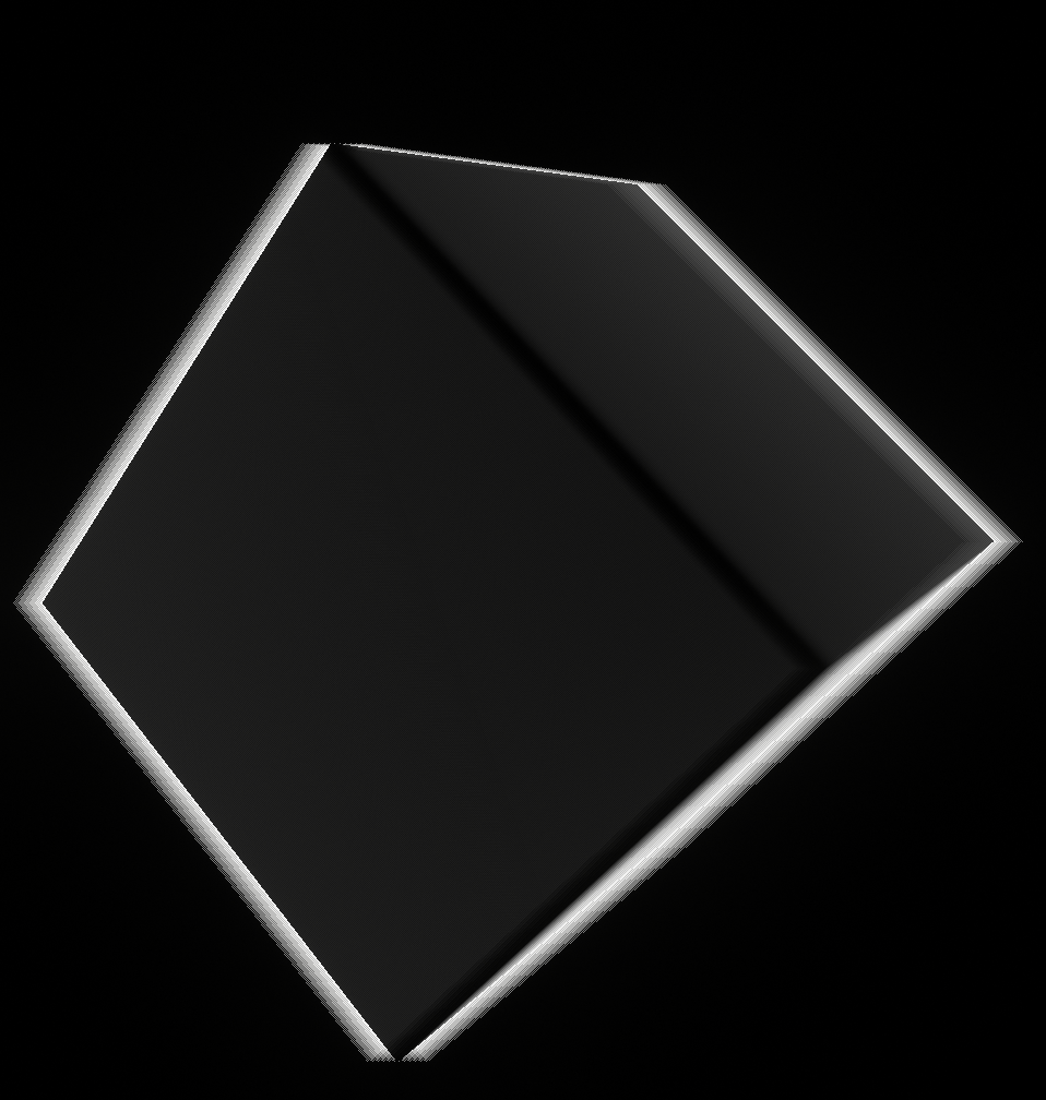
Let’s take a closer look at why the modified depth comparison function is needed. Here are visualizations of the primary direction alpha with the original and modified depth comparison functions. To make the difference more obvious, the weights use a strong horizontal movement on the cube without any background motion.
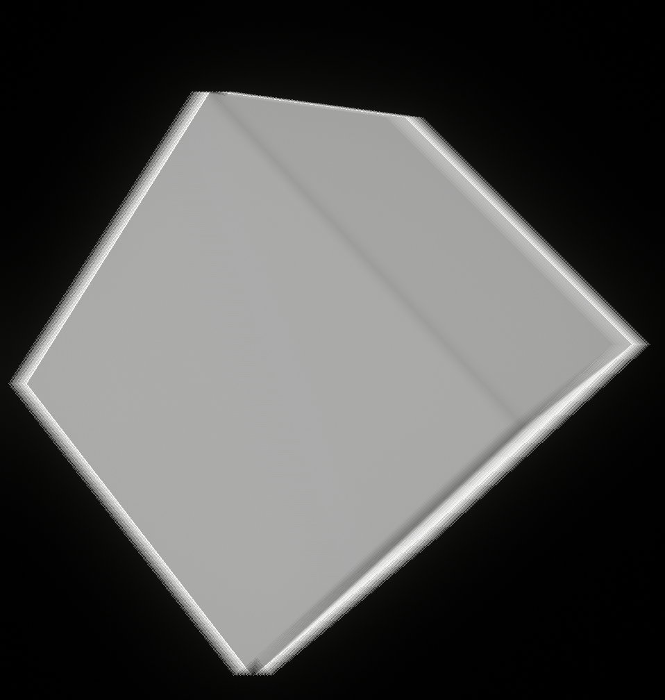
The key insight is that the moving background will produce the same foreground alpha value of 0.5 due to the lack of depth differences. This means that the alpha on the outer edge of the cube blur will be
overwritten by the background’s default alpha of 0.5. Remember that for visualization purposes the background is not moving in the alpha visualization, which is why it has a value of zero there.
By ensuring that foreground alpha is only produced on actual depth differences, we properly separate the foreground and background alphas and ensure
that the max operator works correctly.
And to compare the impact on the final image, here is the final result of using the original comparison function using the synthetic setup from before with strong horizontal foreground and vertical background motion. Notice the discontinuities on the edges between the inner and outer blurs.

For the motion weights, we now need to store per-pixel motion instead of just velocity. To minimize memory bandwidth and cache utilization, I decided to pack both into 32 bit.
Depth remains as a 16-bit float. On a side note, this is when I discovered that HLSL has a f16tof32() intrinsic, which comes in handy for this. Velocity is then packed into the remaining 16-bit
as two 8-bit SNorm values.
Packing and unpacking is done manually in the shader. A recent blog post by Emilio Lopez gives a great overview of the entire topic in case you need a refresher [8].
As a small optimization, the second direction is skipped for very low angles between the primary and secondary direction. This mainly helps with motion caused by camera movement.
I found that even a slightly different secondary direction can still make a noticeable visual difference when an object is rotating. Therefore, the threshold is kept very low at just 5 degrees.
Let’s take a quick peek at the performance impact of using the second direction. The blur cost goes up from ~150us to ~240us with the spinning cube.

L1 and L2 throughputs are slightly increased by roughly 10% and 5% respectively. Cache hit rates are very close with a 2% increase for both L1 and L2. SM throughput is much higher though, almost doubling to 70%. This is probably due to the additional ALU for the separate foreground and background, decoding depth and motion in the shader and the additional motion weight. However, considering that the top bottleneck is still texture throughput, we can assume that the ALU is mostly filling up the memory latency. This version of the shader arguably utilizes the GPU more fully. I did not look into any ALU optimizations, but it doesn’t seem necessary for now.
Post-Filter
Separating filters into multiple passes is an attractive approach since it can multiply the effective sample count. This can enable us to improve quality at a moderate cost. Care needs to be taken however, since the motion blur filter is not trivially separable. Taking inspiration from common depth of field (DoF) approaches, I considered pre- and post-filtering. After some quick experiments with a pre-filter, I dropped the approach because it became very close to just executing the main filter a second time and caused some artifacts in edge cases like corners of moving geometry.
Instead, I switched to a post-filter. When running the post-filter, the main blur pass outputs color and the foreground alpha into a single RGBA16F target. This way, every sample in the post-filter only needs a single texture fetch. In my experience, this tends to be faster on modern GPUs when taking a lot of coherent samples due to putting a lot of pressure on the texture units. Your mileage may vary depending on your hardware, however. Using a 32-bit color and a separate 8-bit alpha might be faster on hardware that is more bandwidth limited or has small caches, so make sure to profile. A similar option for choosing between a single packed or separate smaller textures is discussed in Unreals DoF implementation [9].
The post-filter boils down to a bilateral blur along both sample directions. It is scaled to fill the gaps between the main blur samples. To avoid leaking, it uses point sampling and uses a threshold on the alpha
to discard invalid samples. We know that the alpha gradient is made up of intervals according to the main pass sample count. We take advantage of that by setting the alpha threshold to one over the main pass sample count.
The sample count of the post-filter is scaled according to the covered pixel count. This avoids unnecessary work. In addition, this also balances out the primary and secondary directions, since both
are summed into a single color. For reference, here is the code that computes the blur direction to fill the gaps and computes the sample count. This is executed separately for both directions.
// The blur direction is a radius that we sample in both directions.
// Multiply by half to ensure that neighborhing pixels blur do not overlap.
const float2 blurDirection = 0.5 * blurDirectionMainFilter * mainBlurSampleCountPerSideRcp;

const float coveredPixels = length(dominantMotionNorm * motionNormToPixels) * mainBlurSampleCountPerSideRcp;
const int sampleCountPerSide = min(maxSampleCountPerSide, ceil(coveredPixels));

const float alphaThreshold = 1.0 * mainBlurSampleCountPerSideRcp;
Obviously, we do not want to blur two samples that both have an alpha value of zero. This indicates that the pixels are neither moving nor being blurred over.
However, this causes a small issue. The outer edge of the blur is slightly sharper than intended. This happens because at the end of a gradient multiple pixels have an alpha value of zero due to undersampling.
The post-filter will not blur these.
We can address this by detecting edges. This is done by tracking the maximum alpha from all samples. An edge will have a maximum alpha value of more than zero but below the alpha threshold.
If we encounter an edge, we remove the check that avoids blurring samples that both have an alpha of zero. Since we need the max alpha from all samples, we simply track two versions of the color sum
with different weights and pick the appropriate one at the end. Let’s take a look at the impact of the edge handling in a scene with a strong horizontal blur:


The improvement is subtle but noticeable. The performance impact is relatively minor at ~10us since the shader is relatively light on ALU and register usage. Here’s the relevant code snippets:
// Inside the sampling loop
maxAlpha = max(maxAlpha, colorSample.a);

const bool acceptSample = abs(colorSample.a - centerColor.a) <= alphaThreshold;
const float weight     = acceptSample && !(centerColor.a == 0 && colorSample.a == 0);
const float weightEdge = acceptSample;

colorSum     += weight     * colorSample;
colorSumEdge += weightEdge * colorSample;

weightSum     += weight;
weightSumEdge += weightEdge;

//...

// At the end
const bool isEdge = maxAlpha > 0 && maxAlpha <= alphaThreshold;

colorSum  = isEdge ? colorSumEdge  : colorSum;
weightSum = isEdge ? weightSumEdge : weightSum;

const float4 finalColor = colorSum * rcp(weightSum);
A small performance detail is unrolling the sampling loop as much as possible. We are dealing with dynamic sample counts, so unlike the main blur, the inner loop cannot be unrolled.
The initial implementation had a single loop that started with a negative sample index and directly went over the range \(t = [-1, 1]\). I noticed that performance was subpar,
almost taking as much as the main blur despite simpler logic, only using a single texture fetch per sample, using fewer samples in areas with low velocity and having a smaller working set due to the reduced blur radius.
The solution was to manually unroll the inner loop, starting with sample index zero and iterating over \(t = [0, 1]\). Then we sample at \(t\) and \(-t\).
To avoid duplicating code, I still used a fixed loop with two iterations. This is trivial for the shader compiler to unroll and brought the expected speedup. The cost in my test scene went from ~230us to ~165us.
That’s a pretty good speedup for just changing a couple of lines. Batching memory reads and writes on GPUs can be critical for performance.
Usually, this is where the shader assembly comes in. However, I don’t have access to this on my Nvidia GPU.
A quick Nsight trace reveals that SM throughput is the top bottleneck but still pretty low at
62%. This indicates that we are still suffering from too much latency. Some quick experiments with unrolling the loop by adjusting the sample counts or merging both directions and branching around reads of the second
direction, if unused, did not yield any speedup. However, it is hard to dig into this topic deeper without assembly access and more info on how exactly the hardware works.
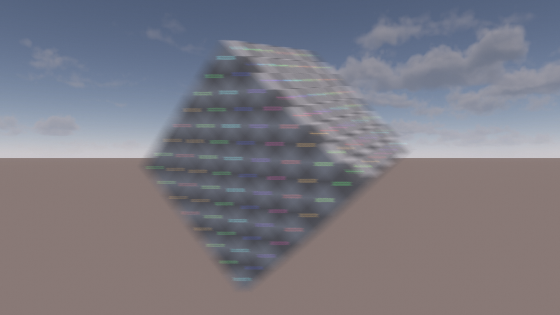
Let’s compare how the postfilter looks in the main scene and compare it to simply doubling the sample count in the main blur.


We can see that in areas of large blur there is less visible undersampling when using the postfilter. As a nice side effect, the postfilter also blurs over the harsh edges between motion tiles. We can tweak the scene to make the difference more obvious. A strong horizontal movement is used and the little colored crosses on the cube texture are made emissive. This makes the scene much less forgiving when it comes to undersampling.

Apart from scenes with bright HDR colors, the post-filter also benefits cases when the blur covers more pixels.
This can happen when a longer blur is desired or the rendering resolution is increased while keeping the blur length constant in screen space.
The post-filter approach is slightly more expensive, however. The motion blur using six samples comes in at ~255us. In addition, the postfilter with up to six samples costs ~170us
for a total of ~425us. Doubling the sample count instead avoids the second pass and increases the blur cost to ~370us.
More Accurate Alpha Computation
There are still some remaining discontinuities in the blur. While digging into this, I discovered that this is caused by mismatches between
the dominant motion velocity and the encountered samples. Let’s consider a simple case: a uniform horizontal movement. The weight and alpha computations should produce a smooth gradient as shown in [3].
But let’s take a look at what happens when the dominant sample direction is twice the size as the actual movement. To clearly demonstrate the issue, I have disabled the postfilter and increased the sample count to 36.

The blur is completely broken. You might wonder why we care about this since this seems like a contrived example. Usually our sample and dominant motion velocities should match.
However, consider what might happen if a single pixel in a neighboring tile is moving significantly faster than the samples we encounter. This can happen in fast rotations.
So what is going on here? Consider how we compute the alpha: we sum up the sample foreground weights and divide by the sample count. The foreground weight is a smooth classification,
but in our simplified case we can conceptualize it as a binary decision. So in the end, we simply count the foreground pixels we encounter. By dividing through the sample count we obtain the ratio of foreground pixels.
At this point, it becomes obvious why this has issues when there is a mismatch between the samples and the sampling direction. Increasing the sampling radius will change the ratio of
foreground pixels.
So how do we fix this? The answer can be found in the same CoD presentation [3] that the motion blur is based on. We need to compute the alpha via a proper scatter-as-gather approach. The presented motion
blur approach uses the aforementioned simplified approach. The depth of field (DoF) uses proper scatter-as-gather, however. I assume this is because the assumption of uniform motion holds in a lot of cases.
Doing something similar for DoF would probably result in far more artifacts because the circle of confusion in a small neighborhood can vary heavily in scenes with a high depth complexity.
Computing proper scatter-as-gather is pretty straightforward. We compute each sample’s alpha as the reciprocal of the area its motion covers. At the end, we divide by the sample count and multiply
with the area we sampled. Every sample covers its own pixel and pixels in two directions according to its velocity \(V\). Therefore the covered area is computed as \(2V + 1\).
The code for this is straightforward. Just remember to apply the mirror filter to the sample alpha as well.
float computePixelArea(float velocityPixels)
{
    return 1.0 + 2.0 * velocityPixels;
}

...

// Inside sampling loop
float sampleAlpha = saturate(foregroundWeight / computePixelArea(sampleVelocityPixels));

// Apply mirror filter to sample alphas before summing them
...

alphaSum += sampleAlpha;

...
// Final alpha computation at the end
const float alpha = saturate(alphaSum * sampleCountRcp * computePixelArea(dominantVelocityPixels);
This fixes the issues in our test case:

In real scenarios, the difference is usually quite subtle. Here is a good example of what kind of improvement you can expect. Note that for demonstration purposes, these images still use a very high sample count instead of the postfilter. Spots where this is relevant will typically suffer from undersampling due to wasting many samples because of the velocity mismatch. We will address this later with further improvements. But let’s stick to what we have established so far to demonstrate the change in isolation:

The performance difference of this change on my system is within the margin of error. The additional ALU should be negligible on most hardware. The only concern is potentially increased register usage.
Half Resolution Rendering
These quality improvements come at a significant performance cost. To counteract the additional cost, I investigated half resolution rendering.
To reduce quality loss as much as possible, we want to keep as much information at full resolution as possible. A very simple approach is to switch to the half-resolution color
when a pixel has received any blur. However, we can do better by retaining the full resolution color in case of a sharp background and a foreground blur.
This naturally fits into our existing foreground/background split.
Half resolution rendering outputs alpha in addition to the color. If there is a blurred background we have to use it. In that case, we already composite foreground and background and output an alpha of one.
In case there is no background, we output the foreground color along with the foreground alpha. This is then used to composite the half resolution blurred foreground
with the full resolution sharp background. The code looks as follows:
float3 finalColor;
float outputAlpha;

if (validBackground)
{
    // We have a blurred background that should replace the full resolution pixels
    // -> compute final color and set alpha to one
    finalColor = lerp(background, foreground, foregroundAlpha);
    outputAlpha = 1;
}
else
{
    // No valid background -> output foreground along with appropriate alpha.
    // Will be lerped after upsample to retain sharp, full resolution background
    finalColor = validForeground ? foreground : centerColor;
    outputAlpha = foregroundAlpha;
}
One potential issue is that naive half-resolution rendering could cause leaking. We already use nearest-neighbor sampling to avoid leaking. We don’t want to accidentally introduce color leaks with this optimization.
Care must be taken when downsampling and upsampling.
There are different options for downsampling. After some experimentation, I landed on using a weighted average that weighs based on the depth distance to the closest pixel.
Basing the downsampling on the closest pixel seemed to work best in my tests. This has additional advantages as well. Leaking is relevant if some pixels are
sharp and some are blurred. If the foreground is blurred, leaking it into the background is irrelevant since it already blurs over it. So the only case we are concerned about is
leaking a blurry background into a sharp foreground. However, a sharp foreground pixel will be ignored during upsampling because we prefer using full resolution data for sharp pixels. This means we can simply
average out the color data.
This is great since it means we don’t need any additional depth or motion data when downsampling. This will come in handy when optimizing later on. In the end, downsampling depth and motion boils down to pretty standard
depth-aware downsampling. Here’s the code snippet for the depth weights:
float MB_computeDownsampleDepthWeight(float referenceDepth, float sampleDepth)
{
    return 1.0 - saturate(abs(referenceDepth - sampleDepth) / g_downsampleDepthRange);
}

float4 MB_computeDataDownsampleWeights(float depth0, float depth1, float depth2, float depth3)
{
    // Replace with max() if you are using reverse-Z
    const float dominantDepth = min(depth0, min(depth1, min(depth2, depth3)));

    float4 weights;
    weights[0] = MB_computeDownsampleDepthWeight(dominantDepth, depth0);
    weights[1] = MB_computeDownsampleDepthWeight(dominantDepth, depth1);
    weights[2] = MB_computeDownsampleDepthWeight(dominantDepth, depth2);
    weights[3] = MB_computeDownsampleDepthWeight(dominantDepth, depth3);

    const float weightSum = dot(weights, 1.0);

    // The dominant depth always has a weight of one, so no need to check for division by zero
    return weights * rcp(weightSum);
}
Leaking must be avoided when upsampling as well. While we used the closest pixel in a 2x2 area for downsampling, we use bilinear interpolation for upsampling. This means the half-resolution
pixel might be behind or in front of the full-resolution pixel. There are four cases we have to consider when it comes to leaking. Most of them are simple, however.
If both pixels are moving, they already blur over each other. If neither pixel is moving, the half resolution alpha is zero and we will simply output the full resolution pixels. If the foreground is moving, it blurs
over the background.
The only interesting case is a moving background and a static foreground. We have to preserve the full resolution edge between foreground and background and avoid leaking
color from the foreground into the background. The latter problem is similar to leaking in DoF. Similar to DoF approaches, leaks can be avoided by weighing the color by its alpha.
This way, the color of static pixels will never contribute.
To retain the edge, we use a standard depth-aware bilateral upsampling. We load full and half resolution depth values and use a smooth depth test. We apply the depth test to the alpha weights. Here’s the code for reference:
float MB_computeUpsampleDepthWeight(float pixelDepth, float sampleDepth)
{
    // Depth weight applied to alpha is responsible for avoiding leakage of
    // blurry background into sharp foreground.
    // Alpha will avoid leaking sharp foreground into blurry background.
    return 1 - saturate((sampleDepth - pixelDepth) / g_upsampleDepthRange);
}

// Alpha weights: bilinear + depth
float weightAlpha0 = bilinearWeight0 * depthWeight0;
float weightAlpha1 = bilinearWeight1 * depthWeight1;
float weightAlpha2 = bilinearWeight2 * depthWeight2;
float weightAlpha3 = bilinearWeight3 * depthWeight3;

// Normalize alpha
alphaWeightSum = weightAlpha0 + weightAlpha1 + weightAlpha2 + weightAlpha3;
{
    const float alphaWeightSumRcp = alphaWeightSum > 0.0 ? rcp(alphaWeightSum) : 0.0;

    weightAlpha0 *= alphaWeightSumRcp;
    weightAlpha1 *= alphaWeightSumRcp;
    weightAlpha2 *= alphaWeightSumRcp;
    weightAlpha3 *= alphaWeightSumRcp;
}

// Some moving corners can end up without any weights.
// In that case disable depth weights.
weightAlpha0 = alphaWeightSum > 0.0 ? weightAlpha0 : bilinearWeight0;
weightAlpha1 = alphaWeightSum > 0.0 ? weightAlpha1 : bilinearWeight1;
weightAlpha2 = alphaWeightSum > 0.0 ? weightAlpha2 : bilinearWeight2;
weightAlpha3 = alphaWeightSum > 0.0 ? weightAlpha3 : bilinearWeight3;

// Multiply color weights with alpha to remove color from pixels that shouldn't contribute.
// Avoids leaking sharp foreground color into blurry background.
float colorWeight0 = bilinearWeight0 * color0.a;
float colorWeight1 = bilinearWeight1 * color1.a;
float colorWeight2 = bilinearWeight2 * color2.a;
float colorWeight3 = bilinearWeight3 * color3.a;

const float colorWeightSum = colorWeight0 + colorWeight1 + colorWeight2 + colorWeight3;
const float colorWeightSumRcp = colorWeightSum > 0.0 ? rcp(colorWeightSum) : 0.0;

colorWeight0 *= colorWeightSumRcp;
colorWeight1 *= colorWeightSumRcp;
colorWeight2 *= colorWeightSumRcp;
colorWeight3 *= colorWeightSumRcp;

const float3 upsampledColor = color0.rgb * colorWeight0 + color1.rgb * colorWeight1 + color2.rgb * colorWeight2 + color3.rgb * colorWeight3;
const float  upsampledAlpha = color0.a   * weightAlpha0 + color1.a   * weightAlpha1 + color2.a   * weightAlpha2 + color3.a   * weightAlpha3;

const float3 finalColor = lerp(fullResColor, upsampledColor, upsampledAlpha);
Let’s take a look at the leaking issues that we avoid by doing this. First let’s compare the upsampling with and without depth weights. This avoids blurry background pixels leaking into the foreground. The comparison is zoomed in and with a bright background to make the difference more obvious.


Here’s a demonstration of the foreground to background leak that the alpha weighing fixes:


And here’s the full scene in full resolution compared to half resolution.


Overall, I’d say the quality is very comparable. The half resolution version has a slightly hazy look due to the half resolution blurring the color in all directions.
On the flip side, it hides some undersampling. The half resolution filtering works as a crude prefiltering step.
One little trick I’m using is to fade out the upsampling alpha when the movement becomes smaller than a half-res pixel. For this, we track the maximum velocity of all samples that influence the pixel.
Here’s the code for reference:
const float halfToFullResFactor = 0.5;
const float maxInfluenceVelocityPixels = maxInfluencedVelocity * constants.velocityNormToPixel * halfToFullResFactor;

// Fading out alpha entirely is a bit oversharpened compared to rendering at full res.
// Clamp to empirically tweaked min alpha.
const float minAlpha = 0.5;

// Minimum alpha when max velocity is full res pixel sized or less.
// Stop modifing alpha when max velocity reaches half res pixel size.
outputAlpha *= remap(maxInfluenceVelocityPixels, 1.0, 2.0, minAlpha, 1.0);
And here is how it would look without this little trick. Compare the sharpness on the green cross in the rotation center. It’s a little exaggerated, but I think the additional sharpness really sells the illusion that we are running the effect at full resolution.

When looking at how this performs we run into an issue, however. A naive implementation of half-resolution rendering has a downsampling pass, followed by the blur and optionally post-filter
and then performs upsampling. However, with this setup the additional cost of down- and upsampling negates most of the time saved by the faster blur passes.
In my case, with all the previously described bells and whistles, the full resolution version runs at ~280us for the main blur and ~175us for the post-filter for a total of ~455us.
The naive half resolution version runs at ~85us for the main blur and ~60us for the post-filter. However, there is an additional downsampling pass at another ~85us and an upsampling pass at ~200us for a total
of ~430us. Barely any gain for all of that effort.
To speed this up, we can output half-resolution data directly from previous full-screen passes. Wether this is possible depends on the exact rendering pipeline, of course.
In my case, I output the depth/motion data from an existing fullscreen depth/motion processing pass that computes camera motion and downsampled depth buffers.
This pass was already responsible for packing depth and motion into a single render target to avoid sampling two different textures to read them [2].
The half resolution output simply replaces the previous output. Quad intrinsics are used for downsampling.
Color is output from the preceding atmosphere composite shader that combines opaque objects with sky, aerial perspective and volumetric clouds using very similar code.
Both shaders are fullscreen compute shaders working on 8x8 tiles per group. In theory, the HLSL spec seems to indicate that quad operations should work as expected when using a 2D
layout that is evenly divisible into quads [10]. However, in the past I ran into issues with this.
So instead, I simply dispatch 1D groups with 64 threads per group and manually swizzle them into quads covering the 8x8 tile. In case you don’t want to
do the bit twiddling yourself, AMD provides a two liner that takes care of this [11].
Upsampling is done directly inside the final composite shader that takes the HDR scene, composites bloom, performs tonemapping and final exposure adjustments and outputs the color into the swapchain.
The additional work in the atmosphere composite shader takes ~20us. The overhead in the depth processing is ~30us.
The initial version of the merged upsampling is more expensive at a ~120us increase. A quick Nsight trace revealed that the bottleneck was texture throughput.
This was surprising to me. I expected this pass to be bandwidth bound. Anyway, there are some easy optimizations. Converting the four depth loads of the
half-resolution samples to a single gather saved a whopping 40us. But we can do better. In most cases, an entire area of the screen will be entirely blurred or entirely sharp.
We can account for this by gathering the half-resolution alpha values first and adding a fast path if they are all zero or one.
If they are all zero, we simply load the full resolution pixel. In case they are all one, we skip loading all depth data and use a single bilinear fetch.
This saves another ~30us over the previous version. This brings the upsampling overhead down to ~50us.
Skipping depth sampling and only sampling either half- or full-resolution color reduces the work that is performed in the upsampling fast path.
It does add latency however, due to dependent texture fetches. This is reflected in the unit throughputs. The top bottleneck shifted to SM throughput, which is still relatively low at 56%.
This seems like a good candidate for overlapping async work or adding more work into the same shader.
Alternatively, we can remove the dependent texture samples by sampling both full- and half-resolution colors for the fast path. Depending on the alpha, we throw away one or both samples.
This reduces latency in the fast path at the cost of increased bandwidth and cache usage. However, this just ends up utilizing more of the GPU resources and is roughly 5-10us faster (3-5%).
VRam throughput of this variant goes up from 35% to 50%. So you probably wouldn’t want to do this in case of going with the aforementioned async option.
These optimizations bring the total cost of the half-resolution version down to ~240us. As a reminder, the full-resolution version took ~455us with the naive half-resolution approach running at ~425us.
One slight complication is that bloom should be run after motion blur. This is especially visible with something extremely bright like the sun. The bloom should match the blurred
shape. I simply use the half resolution color output as the input for the bloom. Note that this forces us to output the proper color even if there is no blur and we end up with an alpha value of zero.
I use the bloom approach from the Jimenez paper [3]. Here the half resolution input is effectively replacing the first downsample. In theory, this may reduce temporal stability due to the lack of a wide filter.
However, with the ubiquitous use of TAA and temporal upscalers I’d expect the input image to be stable enough that this shouldn’t be an issue. I couldn’t test this in my implementation however,
due to the lack of both TAA and problematic content.
As a bonus, this slightly reduces the bloom cost as it gets rid of the first downsample pass. This saves ~60us on my setup. However, my implementation is very unoptimized without sharing any samples via Waveops/LDS.
To be conservative, I checked the numbers when doing a single bilinear tap for the downsample as the upper limit for an optimized implementation. This brings the speedup
for a theoretical, optimized version down to ~35us.
Improving Quality Via Opportunistic Bilinear Interpolation
In theory, bilinear interpolation is attractive since it provides more data per sample. This means we can either achieve a higher quality at the same cost or improve performance by reducing sample counts. However, it introduces leaking. Jimenez observes that bilinear interpolation can be used in the fast path since that is already computing a simple color average [3]. We can go further than that, however. Color leaking only causes relevant artifacts if a pixel is entirely sharp. If a pixel has at least a one pixel blur radius, bilinear interpolation would only slightly extend the blur by another half a pixel. This is irrelevant in practice. With this in mind, we can use bilinear interpolation for color on any tile where the minimum velocity is at least one pixel in size. Depth and motion data remain point sampled to avoid creating unplausible inbetween values. And it is packed into a uint format, so it doesn’t work with hardware filtering in the first place. This enables us to use bilinear sampling on the majority of moving pixels. This even works under complex motion like rotation where we cannot use the fast path.
I decided to improve quality further by doubling sample counts for tiles that are forced to use nearest filtering. The performance overhead of this is manageable thanks to the small number of affected tiles
and relatively cheap filtering cost at half resolution. This approach keeps quality consistently high. I found it sufficient to only apply this to the primary direction.
The primary direction has the larger velocity and is therefore more prone to undersampling, which is where we benefit from the additional samples.
On the spinning cube scene, using linear sampling is only a very minor improvement. The difference is bigger under uniform movement, e.g. when rotating the camera.
Using both linear interpolation and doubling sample counts shows more differences. Some edges are a little bit cleaner and a few areas are a bit smoother.


Where this approach shines is challenging scenarios like rotating thin areas where a lot of samples are rejected. Notice how the dither pattern in the undersampled area on the top is much less visible.

I did not measure any performance penalty for dynamically switching between nearest and linear filtering. Doubling the samples for the nearest filtered tiles costs ~25us. Since both cost and visual impact are relatively minor, this seems like a good fit as an optional feature for higher settings.
Performance
Here’s a table with a breakdown of performance numbers. As mentioned before, this is running at 1080p using 6 samples per direction as a baseline on a GTX 1660 ti with locked clocks.
The timings were taken via DX12 timestamp queries.
All the aforementioned features and optimizations are in use. The single direction variant is listed separately since it’s the most expensive feature variant that is not running in a separate pass like the postfilter.
Even with locked clocks in a static scene and averaging numbers over multiple frames, the timings are not perfectly stable. Therefore, I have rounded everything to the closest 5us.
Note that in addition to what is listed in the table, there is some additional overhead for preparing the data texture containing motion/velocity and depth, as well as the tile motion max filter and dilation.
This should be relatively minor, however.
| Pass | Full Res | Half Res |
|---|---|---|
| Downsample (Merged) | - | 50us |
| Blur One Direction | 220us | 70us |
| Blur Two Directions | 355us | 110us |
| Postfilter | 135us | 60us |
| Upsample (Merged) | - | 40us |
| Bloom Savings | - | -35us |
| Sum: One Direction | 355us | 195us |
| Sum: Two Directions | 490us | 225us |
The difference between the single direction blur at ~220us and the base version we started with that ran at ~160us is due to the extra features. Doubling samples for nearest sampling pixels costs 40us.
The remaining 20us are accounted for by the separate foreground and background sums, the more accurate alpha calculation and outputting a bigger color format with alpha for the postfilter.
I’m pretty happy that the cost of the final half resolution version is just 65us more than what we started with, despite all the quality improvements.
Overall, the half resolution approach pays off for my use case. However, it’s only competitive due to merging down and upsampling into existing shaders to reduce their overhead.
In addition, the savings in the bloom computation play a pretty big role as well and are probably very specific to my exact setup. Even with the merged down- and upsampling steps, it’s easy
for their fixed overhead to eat into the savings. In the end, anything computed at a lower resolution must be expensive enough to warrant
the fixed scaling overhead. The base implementation with a single blur direction and a single pass, for example, would simply not be expensive enough for lower resolution rendering to be worth it.
In terms of scaling, you could easily drop the sample count doubling on nearest filtered tiles to regain a bit of performance. And as mentioned earlier,
doubling the sample count tends to be cheaper than running the extra post-filtering pass. So especially if you are running at half resolution and your blur is not covering too many pixels,
you might be able to get away with dropping the postfilter pass and slightly bumping up the sample count. However, when running at half resolution, decreasing the filtering costs doesn’t even have
that big of an impact due to the fixed overhead of up/downscaling.
Future Work
The biggest topic I did not tackle is how motion blur interacts with anti-aliasing and upscaling. My (latest) hobby renderer is extremely bare bones at the moment and I simply haven’t gotten around to implementing either.
When simply considering anti-aliasing we have to be careful not to introduce leaking. This has been solved before via conservative edge handling [6]. In addition, applying motion blur after AA
can reintroduce aliasing due to alpha edges between sharp foreground and moving background. Not to mention that the depth might be jittered when using TAA. It’s hard to tell how bad these issues might be without
trying it out, however.
When we consider motion blur after upsampling (as recommened by the FSR documentation for example [12]) we don’t have a one-to-one mapping between depth and color values anymore.
This is an issue for the filter itself, as well as up- and downsampling. Perhaps the latter could rely more heavily on color similarity metrics to detect edges that should be preserved.
An alternative would be to do what is commonly done with depth of field and compute the effect before upscaling/AA and temporally stabilize the input data [8]. This would allow
computing the effect at rendering resolution for a more balanced performance/quality option or to go all the way down to half of the rendering resolution.
Conclusion
I hope this post provided you with some useful insights. Perhaps some inspiration to improve on your own motion blur implementation or maybe some just some ideas that can be applied to similar problems. If you have any questions or comments, feel free to reach out via email or X.
References
[1] A Reconstruction Filter for Plausible Motion Blur, McGuire et al. 2012
[2] CryEngine 3 Graphics Gems, Sousa 2013
[3] Next Generation Post Processing in Call of Duty Advanced Warfare, Jimenez 2014
[4] A Fast and Stable Feature-Aware Motion Blur Filter, Guertin et al. 2014
[5] Secrets of CryEngine 3 Graphics Technology, Kasyan et al. 2011
[6] Clustered Forward Rendering and Anti-Aliasing in ‘Detroit: Become Human’, Marchalot 2018
[7] Wave Programming in D3D12 and Vulkan, Lively 2017
[8] The Art Of Packing Data, Lopez 2025
[9] A Life of a Bokeh, Abadie 2018
[10] DirectX-Specs: HLSL Derivative Operations in Compute, Mesh and Amplification Shaders
[11] Optimizing for the Radeon™ RDNA Architecture, Kramer 2020
[12] FSR3 Documentation